
Macroeconomic indicators are traditionally collected with a large lag. This limits their utility in times of high uncertainty. In a pandemic for example, infection rates may accelerate non-linearly (as seen in SIR-models) and are likely to react to variables such as temperature and degree of immunity, many of which remain unknown at the beginning of a pandemic. Nowcasting has been suggested by the Swedish Riksbank (Andersson, Reijer 2015) among others as a tool to make predictions with higher frequency data. Andersson and Reijer use monthly data from surveys, financial markets and similar sources in their nowcasting models to predict Swedish GDP. In this experiment I turned to Google Trends search data to predict movement patterns 1-week-ahead. This time horizon has proven to be relevant in the fast changing landscape of a global pandemic.
In practical terms, what would the utility be of predicting changes in movement patterns? A sharp drop in movement in public spaces can be categorized as a black swan event for affected parties, whether they are retail stores, public transport companies or government agencies. Predicting a sudden change in movement patterns might provide these parties with an opportunity to prepare for this change. Predicted movement patterns can also be used as a leading economic indicator.
Theory
The underlying theory has been advocated for as Narrative Economics by Robert Shiller (2017). But it has featured as a theme in many works without being mentioned by name. Its origins can be traced to the 1930’s when Keynes coined the phrase animal spirits to capture a characteristic of human behavior beyond what was imagined in the classical models of economics.
The assumption is that economic outcomes, to some extent, are a function of the stories and ideas people tell themselves and others. When these stories reach a wide and receptive audience they turn economic behavior into heard behavior. If the narratives that occupy conversations and the minds of people can be measured, they can theoretically be used to predict behavior.
Data
To capture the narrative component I used an R library called gtrendsR which runs the API call to Google Trends so that there’s no need to cURL it manually. The data is slightly unreliable in the sense that Google provides the amount of hits as an index which is calculated in an unknown black box of magic. The index does however seem to measure changes in search trends over a shorter time horizon reasonably well.
The query used in Google Trends was covid and virus. As the interest in Covid-19 rises, people are expected to go online to search for information about the virus or the situation as it unfolds which registers in the index. This variable is countercyclical and should be negatively correlated with movement patterns.
A procyclical variable was used as well. For this variable my query was snälltåget and sj which are the main operators of long distance trains in Sweden. The assumption here is that people on average go online and search for train tickets 1 week ahead of departure. This variable should be positively correlated with movement patterns.
For data on movement patterns I used Google Mobility Report. It was launched in the infancy of the Covid-19 pandemic to track changes in movement patterns. It calculates changes from the same days baseline categorized by country, sub region and type of location/activity (retail and recreation, parks, homes etc).
Model
One of the problems with applying a simple linear regression model is that time series data are likely to be autocorrelated which will express itself as covariance between residuals. One way of resolving this is to model the residuals as an ARIMA-process. I ended up with a (1,1,0) process here. So the model used will be a linear regression with ARIMA errors. Sometimes referred to as ARIMAX, where the X denotes an external regressor.
The equation:
$Y_t = B_1X_{1t} + B_2X_{2t} + n_t$ where $n_t = \phi n_{t-1} + \epsilon _t$ is the ARIMA error term. Notations for differencing are missing.
In the model, narratives are spread at time t and have an effect on economic behavior at time t+1. Having input variables lagged at t+1 allows the use of an external regressor as fresh input for 1-step-ahead predictions in an ARIMAX model.
R code
Libraries:
library(tidyverse)
library(gtrendsR) # for Google Trends API calls.
library(fable) # tidyverse compatible replacement of the forecast package.
library(feasts)
library(tsibble)
library(lubridate) # to help with some weekly time series strangeness.
These were the inputs in the Google Trends API call.
query <- c("covid", "virus")
query2 <- c("snälltåget", "sj")
date <- c("2020-03-01 2021-01-15")
I wrote a function which loops along the query vectors and outputs the mean of hits (index of times searched) in a data frame. This allows for easy experimentation with different search queries and explorative data analysis.
search_se <- data.frame()

search_se_mean <- function(query) {
  for(i in seq_along(search)) {
    print(search[i])
    search_se <- rbind(covid_se,
                      gtrends(keyword = search[i],
                              geo = "SE",
                              time = date)[[1]])
  }

search_se_mean <- search_se %>%
  mutate(week = yearweek(date, week_start = 1)) %>%
  group_by(week) %>%
  summarise(hits = mean(hits))
}

gtrends_nar <- search_se_mean(query)
gtrends_beh <- search_se_mean(query2)

gtrends_se <- gtrends_nar %>%
  full_join(gtrends_beh, by = "week", suffix = c("_nar", "_beh"))
Plotted together:
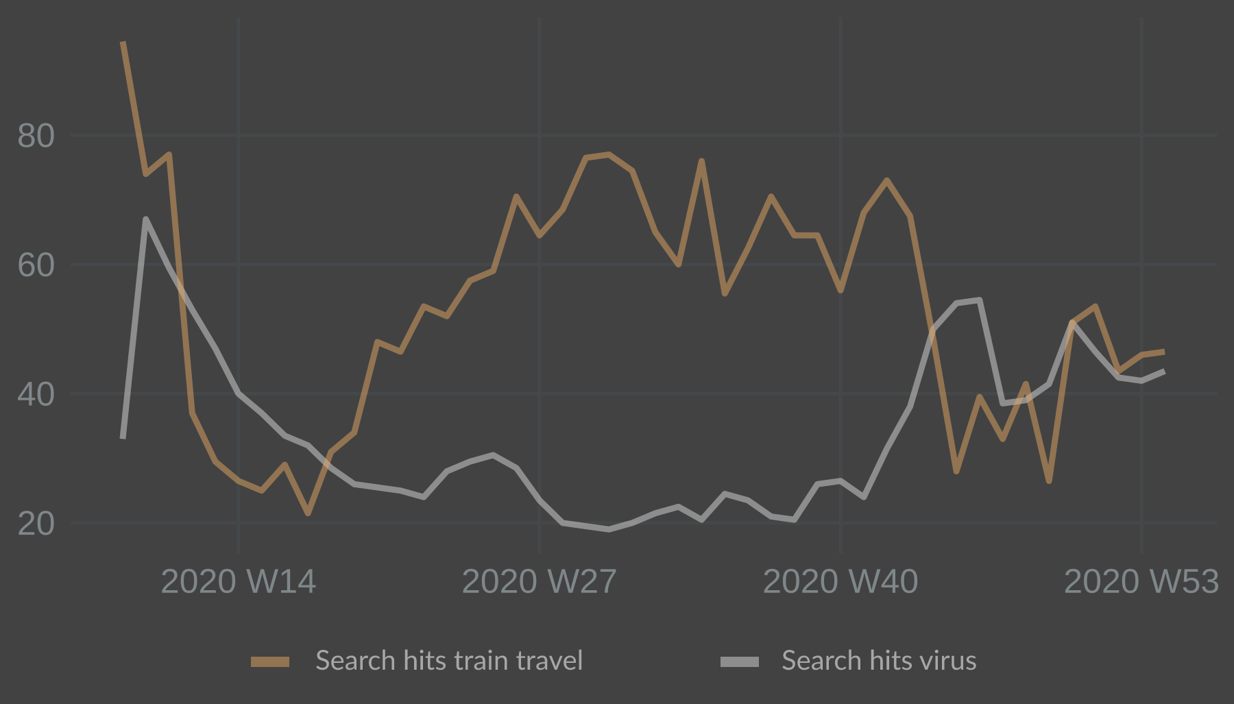
Hits for train travel dropped sharply, as one would expect, and then rebounded over the summer. Hits for the virus jumped up initially but dropped surprisingly fast. Lower levels over the summer was in line with a lower spread of the virus. The index jumped up again in the autumn of 2020, in line with a rising spread of the virus. This inverse relationship between the train travel and virus narrative predictors made intuitive sense and looked promising.
The next step was to find out if the predictors had any explanatory power on the leading indicator: movement patterns.
The movement data is available at https://www.google.com/covid19/mobility/ I used the .csv-file for global data and did the filtering for my region of interest in R.
Once it’s loaded, the following code will filter for the target country with country_region_code. I filtered for sub_region_1 = "" in order to capture data for all of Sweden. The data is then transformed into weeks. Note that data for retail_and_recreation_percent_change_from_baseline was used. The movement patterns being predicted are in retail and recreation areas.
gmr_se <- gmr %>%
  mutate(date = as_date(date)) %>%
  filter(country_region_code == "SE",
         sub_region_1 == "",
         date >= "2020-03-01" & date <= "2021-01-17") %>%
  select(date, retail_and_recreation_percent_change_from_baseline) %>%
  mutate(week = yearweek(date, week_start = 1)) %>%
  group_by(week) %>%
  summarise(across(everything(), list(mean))) %>%
  rename(
    "retail" = retail_and_recreation_percent_change_from_baseline_1) %>%
  select(week, retail)

df_se <- gtrends_se %>% # join data sets together
  left_join(gmr_se)

df_se$retail <- df_se$retail + 100 # for potential differencing and log transformations
Regressions and scatter plots:
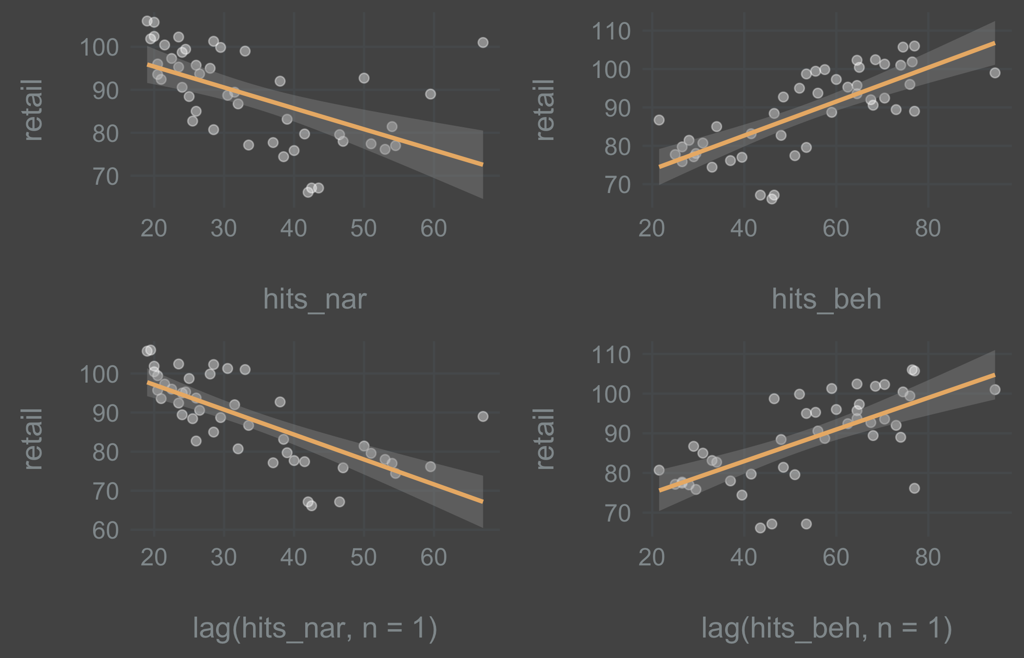
Inspecting the plots revealed that there was a linear relationship between the variables. The virus search variable did well with 1 lag, while the train ticket search did better without a lag. This will likely depend a lot on the search queries used and on the reliability of Google’s black box data. For the purpose of this experiment I stuck with the theory in order to be able to predict 1-step-ahead and continued with lagged variables.
Next, preparing the data for model fitting.
val_weeks <- 15 #15 weeks for validating the models

df_se_index <- df_se %>%
  mutate(index = seq_along(1:nrow(.)),
    type = if_else(index > max(index) - val_weeks,
    "validation", "training"),
    hits_nar_lag = lag(hits_nar),
    hits_beh_lag = lag(hits_beh))

tsibble_se <- as_tsibble(df_se_index, index = index) # as time series tibble

tsibble_se_train <- tsibble_se %>%
  filter(type == "training")

tsibble_se_val <- tsibble_se %>%
  filter(type == "validation")
Computing both the TSLM and the ARIMAX (1,1,0) model to see if it makes sense to model the residuals as an ARIMA-process.
fit_tslm <- tsibble_se_train %>% # fit the model on the training data
model(TSLM(retail ~ hits_nar_lag + hits_beh_lag))
fc_tslm <- fit_tslm %>% # forecast with the validation data
forecast(new_data = tsibble_se_val)
fit_arimax <- tsibble_se_train %>%
model(ARIMA(retail ~ hits_nar_lag + hits_beh_lag + pdq(1, 1, 0)))
fc_arimax <- fit_arimax %>%
forecast(new_data = tsibble_se_val)
rmse_tslm <- round(accuracy(fit_tslm)[, 4], digits = 2) # extract RMSE
rmse_arimax <- round(accuracy(fit_arimax)[, 4], digits = 2) # extract RMSE
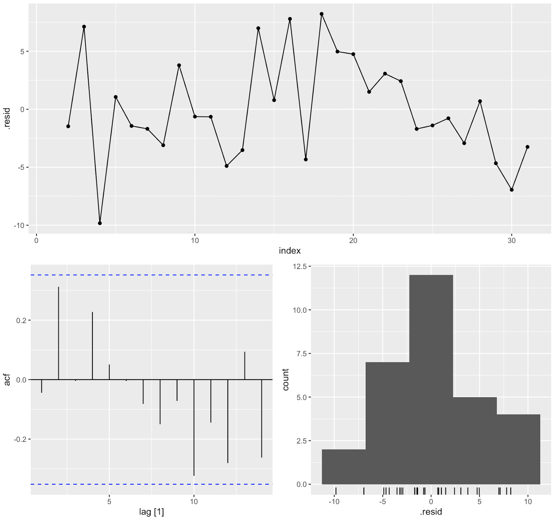
fit_tslm %>% gg_tsresiduals()
The patterns at index > 18 or so didn’t look like a white noise-process. This shows up in the ACF plot as well, even though the spikes aren’t significant. The takeaway is that modeling the residuals as an ARIMA-process might prove useful.
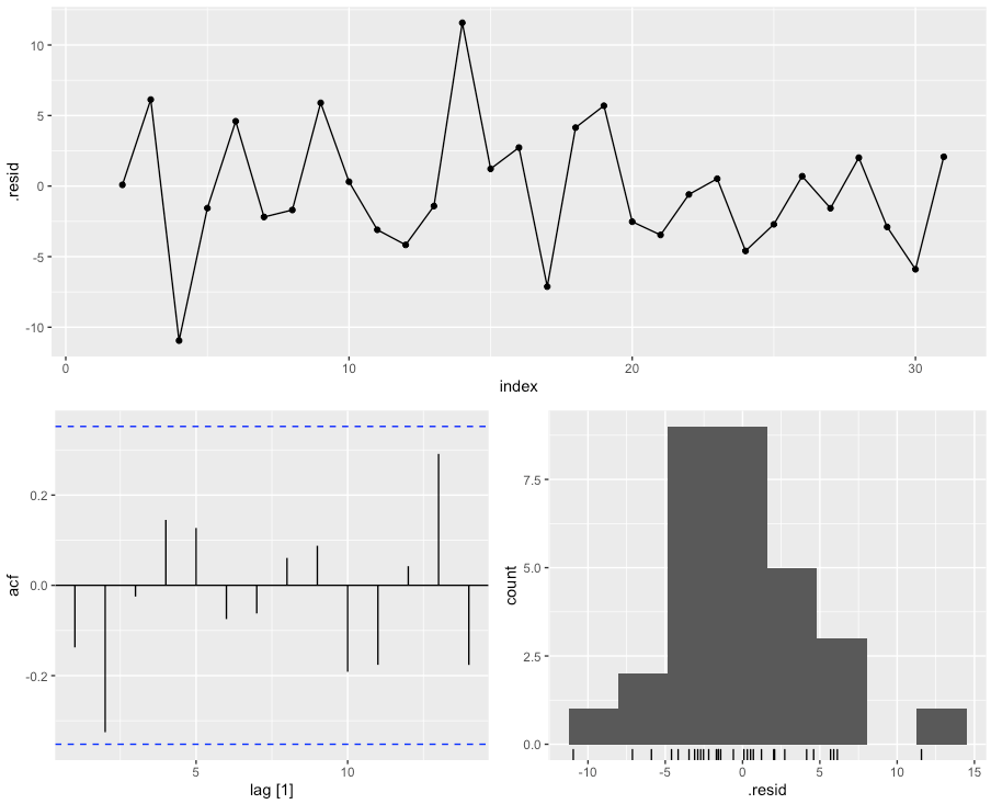
Fitting the ARIMAX-model below. Evaluating the residuals, they looked more like a stationary white noise process. No significant spikes.
Plotting the models and forecasts produced with Fable:
tslm_plot <-
  tsibble_se %>%
  mutate(color = if_else(type == "training", "#7e828c", "#7e828c")) %>%
  ggplot(aes(x = index, y = retail)) +
  geom_line() +
  autolayer(fc_tslm, alpha = 0.5, color = "#aa332c") +
  geom_line(aes(color = color), alpha = 0.8) +
  geom_line(aes(y = .fitted, color = "#aa332c"), data = augment(fit_tslm)) +
  labs(
    title = "TSLM model",
    subtitle = paste0("RMSE = ", rmse_tslm)) +
  scale_color_identity()

arimax_plot <-
  tsibble_se %>%
  mutate(color = if_else(type == "training", "#7e828c", "#7e828c")) %>%
  ggplot(aes(x = index, y = retail)) +
  geom_line() +
  autolayer(fc_arimax, alpha = 0.5, color = "#aa332c") +
  geom_line(aes(color = color), alpha = 0.8) +
  geom_line(aes(y = .fitted, color = "#aa332c"), data = augment(fit_arimax)) +
  labs(
    title = "ARIMAX model",
    subtitle = paste0("RMSE = ", rmse_arimax)) +
  scale_color_identity()

grid.arrange(tslm_plot, arimax_plot, nrow = 2)
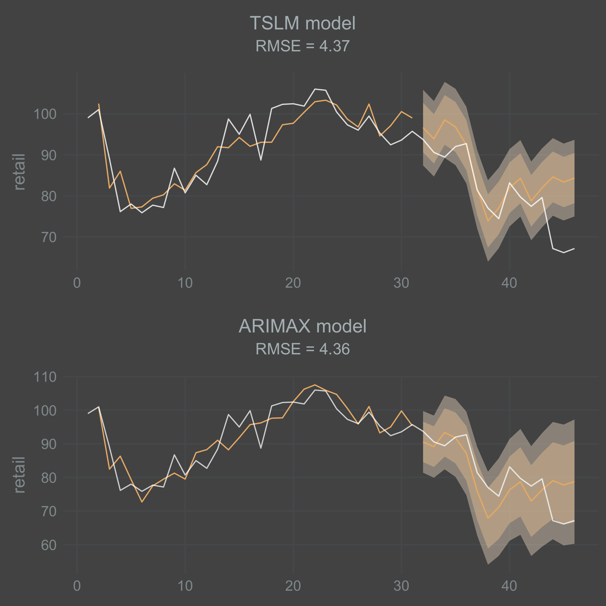
I’m a bit surprised that the fitted TSLM model performed in parity with the ARIMAX model. I think this might vary a lot depending on the data you end up with. Both models do a decent job on the training data. But they both do a poor job at forecasting the sharp drop in movement that occurs at the end of the time series. I should point out that the ARIMAX model is forecasting the AR(1)-process recursively here. Consequently, there is a mean reversion and it looses its effect over time.
Since I’m interested in the 1-step-ahead forecast, I wrote the loop below to capture what that looks like on the validation data. The point here is to capture the direct 1-step-ahead forecast instead of a recursive forecast, and thereby utilize the full potential of the ARIMAX-model.
tsibble_se_loop <- data.frame()
direct_pred <- data.frame()
index <- 15:nrow(tsibble_se)
val_weeks = 1
for(i in index) {
tsibble_se_loop <- df_se %>%
mutate(index = seq_along(1:nrow(.)),
hits_nar_lag = lag(hits_nar),
hits_beh_lag = lag(hits_beh)) %>%
as_tsibble(., index = index) %>%
filter(index < index[i]) %>%
mutate(type = if_else(index > max(index) - val_weeks,
"validation", "training"))
# Save the training data
tibble_train_loop <- tsibble_se_loop %>%
filter(type == "training")
# Save the validation data
tibble_val_loop <- tsibble_se_loop %>%
filter(type == "validation")
fit_arimax <- tibble_train_loop %>%
model(ARIMA(retail ~ hits_nar_lag + hits_beh_lag + pdq(1, 1, 0)))
fc_arimax <- fit_arimax %>%
forecast(new_data = tibble_val_loop)
fc_arimax <- as_tibble(fc_arimax) %>%
select(index, .mean)
direct_pred <- rbind(direct_pred, fc_arimax)
}
direct_pred <- as_tsibble(direct_pred, index = index)
arimax_direct_plot <-
tsibble_se %>%
mutate(color = if_else(type == "training", "#7e828c", "#7e828c")) %>%
ggplot(aes(x = index, y = retail)) +
geom_line() +
geom_point(aes(x = index, y = .mean), color = "#aa332c", fill = "#aa332c", size = 2, alpha = .8, data = direct_pred) +
autolayer(direct_pred, alpha = 0.8, color = "#aa332c") +
labs(
title = "ARIMAX model",
subtitle = "with 1-step-ahead direct forecast") +
scale_color_identity() +
theme(
axis.title.x = element_blank()
)
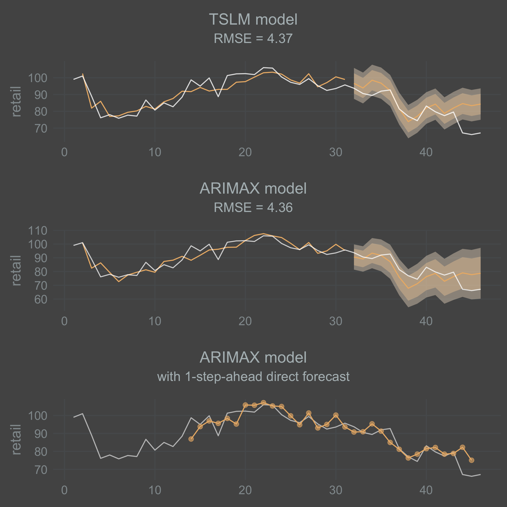
grid.arrange(tslm_plot, arimax_plot, arimax_direct_plot, nrow = 3)
Conclusion
The direct 1-step-ahead ARIMAX forecast does a little better than both the TSLM and the ARIMAX recursive forecast at self-correcting for the last drop off in movement. But still, it essentially fails to predict that last drop 1 week ahead. Leaving that aside, the level of predictive power in the model is surprising considering its simplicity. What I take away from this experiment is that with a bit of fine-tuning and perhaps added complexity it is possible to predict a leading economic indicator with high-frequency narrative data.
The fact that the virus search variable did better with 1 lag as predicted while the train ticket search variable did worse is interesting. It might indicate that people don’t plan ahead when traveling by train or that train travel has an added element of spontaneity in times of high uncertainty when there is already a pent up demand for travel.
For future experiments it would be interesting to explore a machine learning technique with a larger and more varied narrative data set. The statistical rigor offered by conventional techniques are not as relevant in a forecasting model as they are when exploring a casual relationship.
References
Andersson, Michael K. and Reijer, Ard H.J. (2015), “Nowcasting”, Sveriges Riksbank Economic Review, 2015:1, Sveriges Riksbank, pp. 75-89.
Shiller, J.R. (2017) Narrative Economics. NBER Working Paper, No. 23075.